7.7 Launching the ArchRBrowser
One challenge inherent to scATAC-seq data analysis is genome-track level visualizations of chromatin accessibility observed within groups of. Traditionally, track visualization requires grouping the scATAC-seq fragments, creating a genome coverage bigwig, and normalizing this track for quantitative visualization. Typically, end-users use a genome browser such as the WashU Epigenome Browser, the UCSC Genome Browser, or the IGV browser to visualize these sequencing tracks. This process involves using multiple software and any change to the cellular groups or addition of more samples requires re-generation of bigwig files etc., which can become time consuming.
For this reason, ArchR has a Shiny-based interactive genome browser that can be launched with a single line of code ArchRBrowser(ArchRProj). The data storage strategy implemented in Arrow files allows this interactive browser to dynamically change the cell groupings, resolution, and normalization, enabling real-time track-level visualizations. The ArchR Genome Browser also creates high-quality vectorized images in PDF format for publication or distribution. Additionally, the browser accepts user-supplied input files such as a GenomicRanges object to display features, via the features parameter, or genomic interaction files that define co-accessibility, peak-to-gene linkages, or loops from chromatin conformation data via the loops parameter. For loops the expected format is a GRanges object whose start position represents the center position of one loop anchor and whose end position represents the center position of the other loop anchor.
To launch our local interactive genome browser, we use the ArchRBrowser() function.
When we start, we see a screen that looks like this:
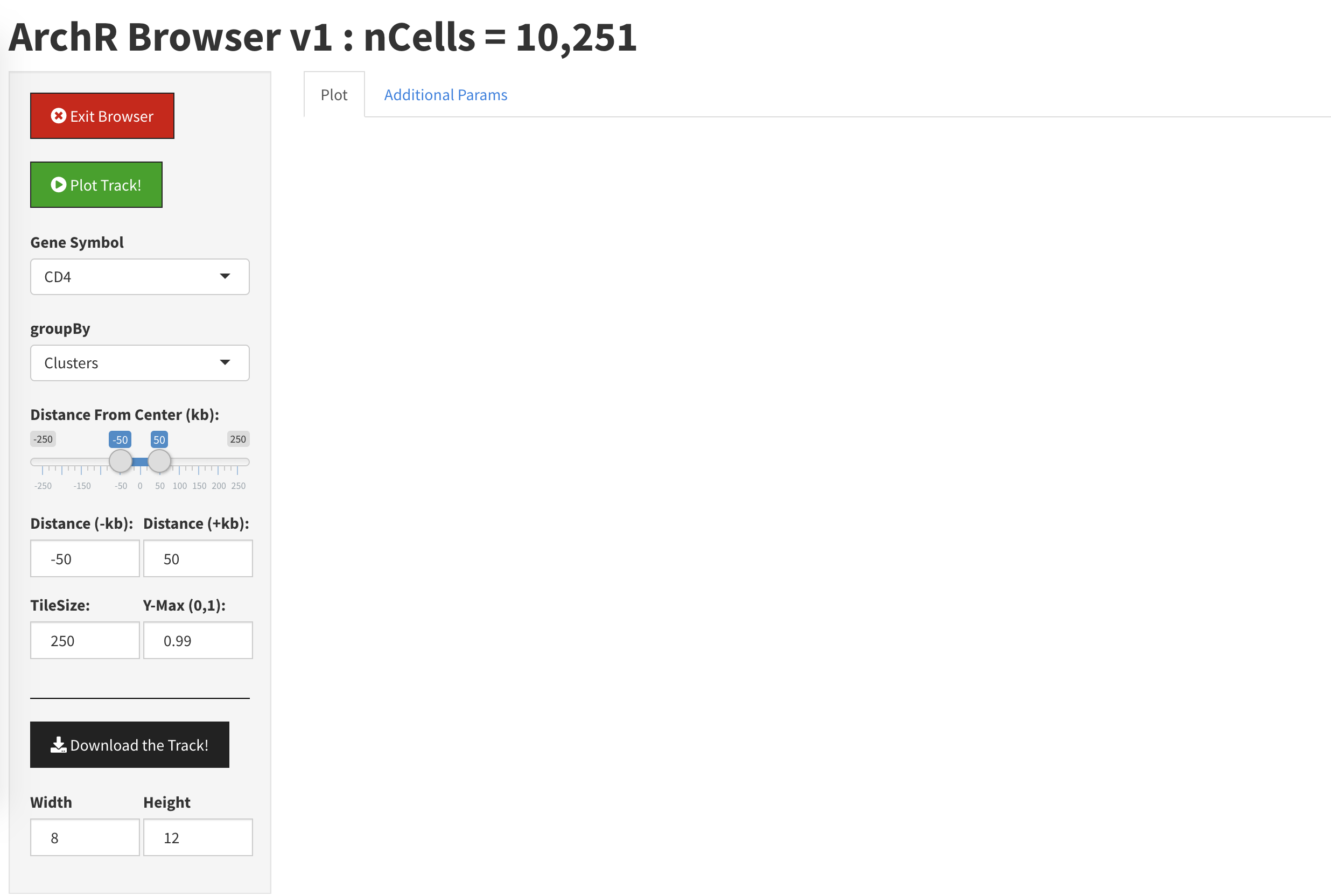
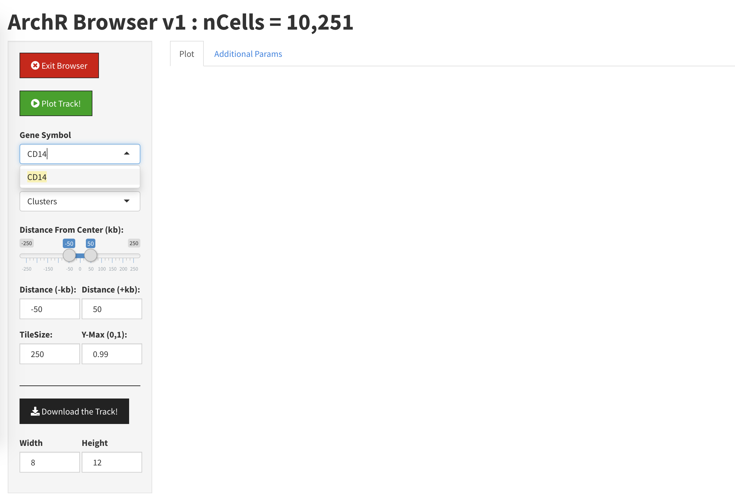
By selecting a gene via the “Gene Symbol” box, we can begin browsing. You may need to click the “Plot Track” button to force your browser session to update.
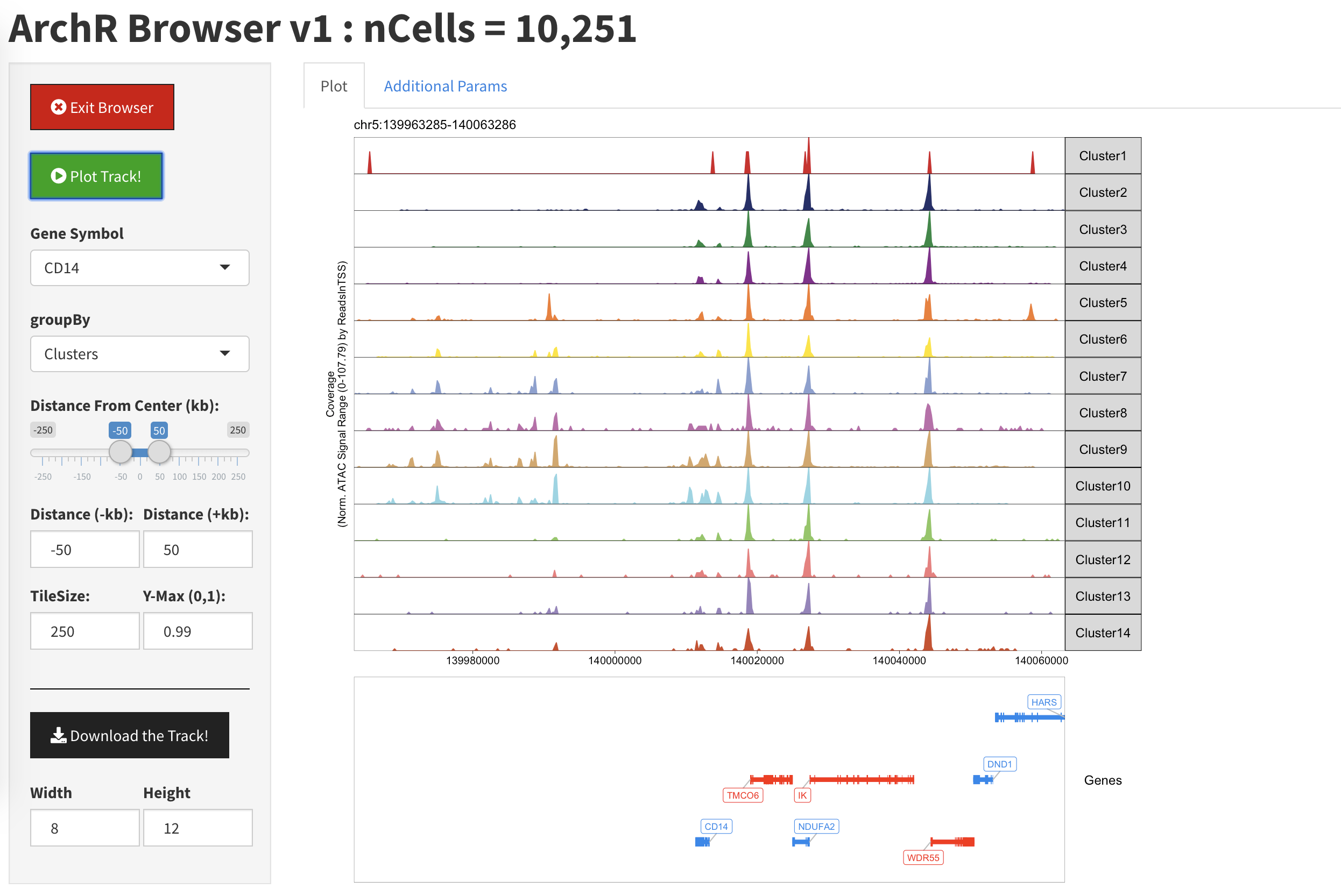
Once we have plotted a gene locus, we see a single track representing each of the clusters in our data.
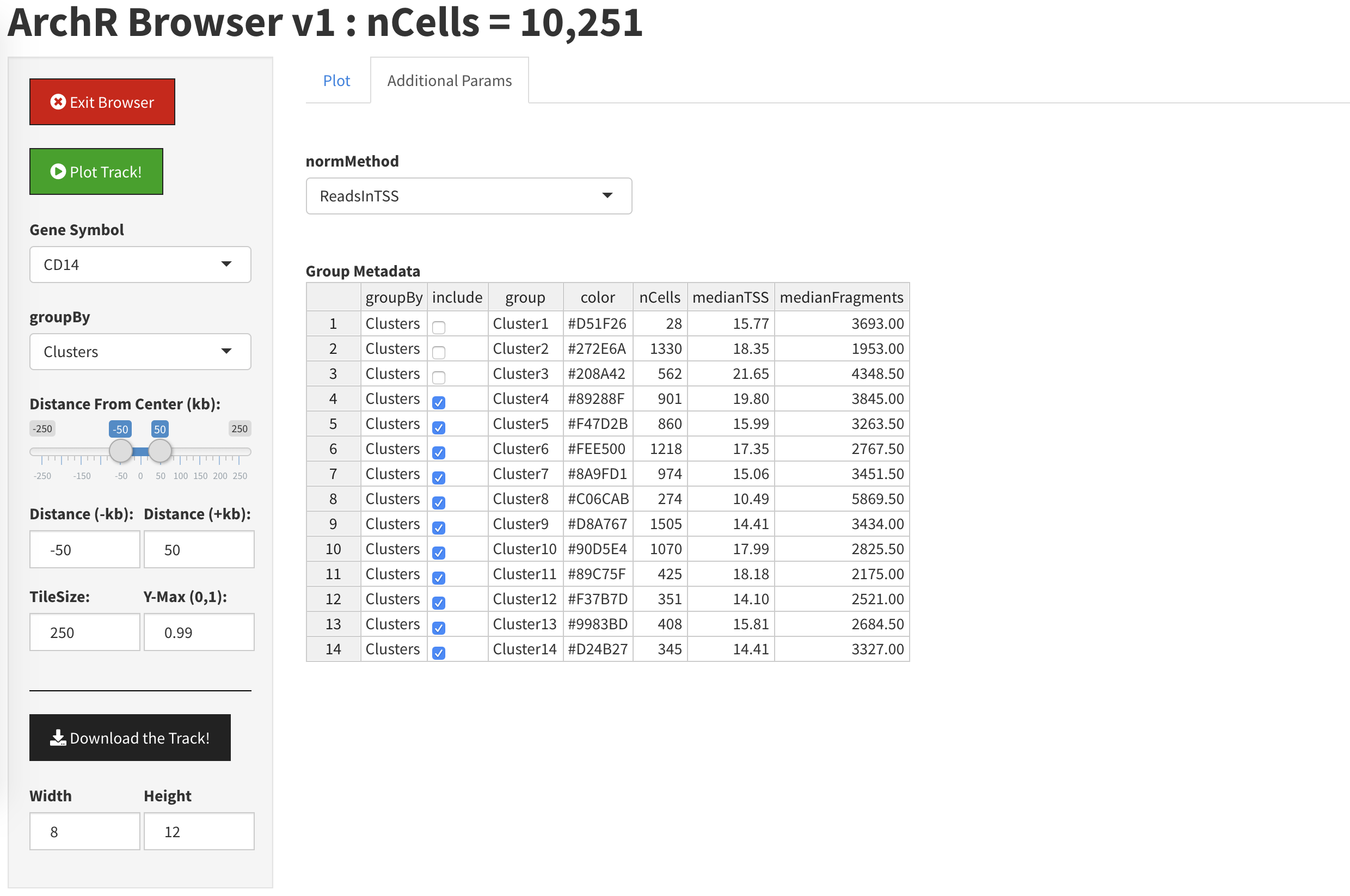
If we click the “Additional Parameters” tab, we can specify which clusters to display and which to hide.
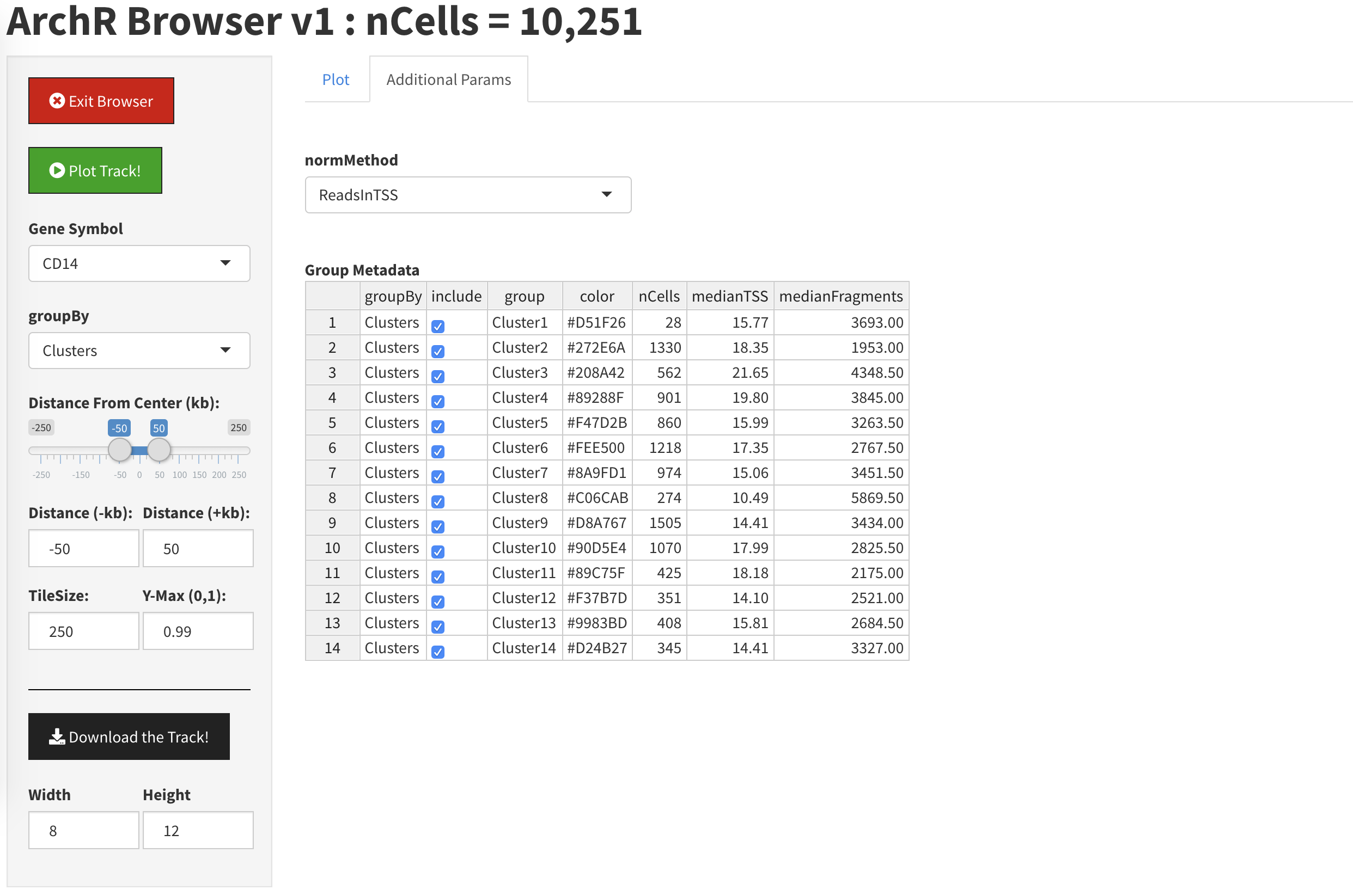
By unclicking the check boes next to Clusters 1, 2, and 3, we will remove them from the plot.
When we return to the “Plot” tab, we should see an updated plot with Clusters 1, 2, and 3 removed. Again, you may need to click the “Plot Track” button to force your browser session to update.

At any point, we can export a vectorized PDF of the current track view using the “Donwload the Track” button.